Acoustic imaging (basics)

In this section, we will explain some basics of acoustic theory to understand the propagation of acoustic waves and the echographic process.

Propagation of acoustic waves

In this section, we will define the different types of acoustic waves and some basic equations and properties of the propagation of acoustic waves.

Wave types

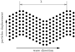
An acoustic wave is a perturbation of the local state without displacement of the global state. Acoustic waves are periodic, their spatial periodicity is given by the wavelength λ. Consider a medium at rest such as on Fig. 1, where particles are represented by the dots. Such a periodic structure represent a metal for example. When an acoustic wave propagate in this medium, the particles will have a local displacement.

There are two types of acoustic waves : longitudinal waves (Fig. 2) also named P waves, and transverse waves (Fig. 3) also named SH or SV waves. Longitudinal waves are compressional waves, in which the direction of displacement of the medium particles is the same than the direction of propagation of the wave. Transverse waves are shear waves, their direction of displacement is then perpendicular to the direction of propagation of the wave. In a fluid, such as water, only longitudinal waves can propagate. In the biological tissues composing the human body, the shear modulus is very small, hence it can be considered as a fluid and only longitudinal waves will be generated.

In the rest of the document, we will only consider longitudinal waves.

Mathematical formulation

In acoustics, a fluid medium is described by two mechanical parameters: the mass density ρ and the bulk modulus κ. The bulk modulus relates the change of volume of a medium to the isostatic pressure applied on it. The velocity of the acoustic wave c is:

$c=\sqrt{\dfrac{\kappa}{\rho}},$

for example, for water we have: ρ = 1000 kg.m⁻³, κ = 2.19 MPa and c = 1480 m.s⁻¹.

The mathematical formulation is obtained by solving the Helmholtz equation, for example, the acoustic pressure p(x,t) can be expressed as:

$p\left(x,t\right)=\left(A^{+}e^{i kx}+A^{-}e^{-i kx}\right)e^{-i \omega t},$

$A^{+}e^{i kx}$ is a wave of amplitude A⁺, propagating towards the positive x, $A^{-}e^{-i kx}$ is a wave of amplitude A⁻, propagating towards the negative x. $k=\dfrac{\omega}{c}$ is the wavenumber, ω = 2πf the angular pulsation and f the frequency.

When we make an echographic image, we are interested only in the intensity of the wave:

$I=\dfrac{1}{2}\Re\left[p\left(x,t\right)v^{*}\left(x,t\right)\right],$

where v(x,t) is the velocity of the particle, and v^* represents the complex conjugate of v. It can be shown with Euler’s equation that the intensity is directly proportional to the square modulus of the pressure.

Refraction and diffusion of acoustic waves

When an acoustic wave passes from a medium (0) to a second medium (1), a part of the wave is reflected and the other part is transmitted through the interface. When the interface is flat from the point of view of the wave, we have refraction (it is a quasi one dimensional problem, because the wave is reflected in only one spatial direction). When the wave sees the curvature of the interface, the wave is scattered on all the directions of the space, we then talk about diffusion.

Refraction of a wave

We consider an incident wave $\phi_{inc}$ normal to an interface, the reflected $\phi_{R}=R\phi_{inc}$ and the transmitted $\phi_{T}=T\phi_{inc}$ waves are also normal to the interface (Fig. 4). R and T represent the reflection and transmission coefficient, respectively. By solving this problem, we show that:

$R=\dfrac{Z_2-Z_1}{Z_2+Z_1},$

where Z_i = ρ_ic_i is the acoustic impedance of the medium i.

If we consider for example the reflection of a wave at an interface between water (ρ₀ = 1000 kg.m⁻³, c₀ = 1480 m.s⁻¹) and a muscle (ρ₁ = 1070 kg.m⁻³, c₁ = 1590 m.s⁻¹), the reflection coefficient is equal to 69.10⁻³, so only 7% of the pressure is reflected. In the case of an interface between water and bone (ρ₁ = 2175 kg.m⁻³, c₁ = 4000 m.s⁻¹), then nearly 70% of the incident wave is reflected. Echoes due to bones are much more higher than the ones due to muscles.

Scattering of a wave

Scattering occurs when a wave hits small or pointlike objects (Fig. 5). The scattered wave equation is much more difficult to derive, compared to the reflected wave equation seen above. However, the scattered wave goes in every direction of space : it follows that its amplitude decreases rapidly with the distance from the object.

Attenuative media

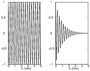
The human body is an attenuative medium, meaning that the amplitude of an ultrasound wave propagating in a such medium decreases along its direction of propagation. Mathematically, the propagation of waves in this kind of medium is written as:

$p\left(x,t\right)=\left(A^{+}e^{i kx}e^{-\alpha x}+A^{-}e^{-i kx}e^{\alpha x}\right)e^{-i \omega t}$

Fig. 6 shows the difference between amplitude profiles for a wave propagating in a non-attenuative (left) and an attenuative medium (right). When we perform acoustic imaging in the human body, we must gradually amplify the received signal in order to accurately convert the analogical signal into a digital signal. Indeed, if the amplitude of the signal is smaller than the precision of the ADC, we can’t measure it (see Appendix). Classically, we apply Time Gain Compensation (TGC) to the received signal in order to keep a convenient amplitude level. An example of this kind of treatment is presented in Fig. 7, where it is applied to the attenuated signal on the right side of Fig. 6.

Transducer

A transducer is an acoustic sensor converting electric power to mechanical power and conversely. If an electric signal is applied to the transducer, it will generate acoustic waves (like a speaker), and if an acoustic wave deforms it, the transducer generates an electrical signal (like a microphone).

In order to have a correct radial precision in acoustic imaging, the acoustic wave must be focused on one point. This can be done using two kinds of technologies: focused transducers and transducer arrays.

Focused transducer

This kind of transducer has a spherical shape, so the emitted acoustic wave is naturally focalised to the center of the sphere (Fig. 8). The area of the focal spot is an ellipse, the value of l and L can be approximated by:

$l=\dfrac{\lambda R}{2r},$

$L=15\left(1-0.01\theta\right)l$

When the angle θ is large, the ellipse elongation is small. When we do acoustic imaging, we want the minor axis l to be as small as possible to increase the radial precision. Moreover, we want the major axis L to be high, because the echo of an object outside of this ellipse will be too small to be measured. So we have to make a compromise between l and L.

At the near field (depending on λ and r) of the transducer, the acoustic pressure is too chaotic so we can’t do acoustic imaging in the near field of this kind of transducer.

Transducer arrays

When transducers are assembled in an array, the size of each transducer is generally small compared to the wavelength, so they emit spherical waves. If all the transducers emit a wave at the same time, the array will emit a plane wave. With a proper delay applied between the emission of each transducer, it is possible to generate a focused acoustic wave (Fig. 9). This delay can easily be computed, indeed, by knowing the distance between each transducer, in order to determine a delay that consists on having all the waves generated by each transducers arriving exactly at the same time to a given point in space. By doing this the waves interfere coherently near this point (high pressure) and incoherently everywhere else (low pressure).

With a transducer array, it is possible to focalise at different points at the same time, so acoustic imaging can be faster with this and it does not need a motor to image a plane. However they are much more expensive than a simple focused transducer and the electronic is much more complicated to drive a transducers array.

Signal Processing

In this section we introduce the Fast Fourier Transform (FFT) and present a basic signal processing technique to improve an echographic signal.

Fast Fourier Transform

The Fourier transform is a transformation that express a function of a given dimension as a function of another dimension. Classically, a time-dependent signal is expressed as a function of the frequencies. In acoustic we also apply Fourier transforms to a space-dependent signal, so the transform is a function of the wavelength. The Fourier Transform S of a real signal s is complex, ℜ(S) is an even function and ℑ(S) is odd.

The FFT is an algorithm that calculate the Fourier transform of a signal very fast, the number of points of the signal must be a power of 2. The FFT of a signal is a periodic function with a periodicity equal to the frequency sampling of the initial signal. Classically, the FFT algorithm returns the Fourier Transform for positive frequencies. Due to the periodicity of the FFT, the second half of the signal is the negative frequency part.

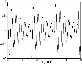
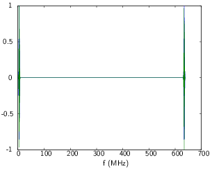
Consider a time signal sample at frequency f_e = 640 MHz composed of N=1024 points (Fig. 10). If you keep only the positive frequencies, the frequency vector corresponding to the FFT ranges from 0 to $f\_e\dfrac{N-1}{N}$. An octave is given by linspace(0,fe*(N-1)/N,N). The FFT of the time signal keeping the positive frequencies is presented on Fig. 11.

If one wants to filter the signal, it is more convenient to consider the negative frequencies, because if you want to filter a signal between x and y MHz, you must put to 0 all frequencies except the points between x and y MHz as well as the points between -x and -y MHz. In this case, the frequency vector is given by linspace(-fe/2*(N-1)/Nfe/2,N) and you must put the second half of the FFT signal at the beginning. To do that you must create a new vector of the same size than the FFT signal, and doing for example: S2(1:N/2-1)=S(N/2+2:end) and S2(N/2:end)=S(1:N/2+1). Then you obtain the signal presented on Fig. 12.

The real and imaginary part of the FFT are presented on Figs. 11 and 12 and are divided by their maximum amplitude to have readable graphics.

If one wants to know the central frequency of a transducer, you must take the modulus of the FFT of an echo of the transducer. The central frequency is the frequency where the modulus has the higher value.

Hilbert transform

The Hilbert transform is useful for signal processing in echographic imaging, because with this transformation we can access to the envelope of a given signal. The Hilbert transform can easily be determined with the FFT. Indeed, if you calculate the FFT of a signal and put all the negative frequencies to 0 and do an IFFT (Inverse Fast Fourier Transform), then you have the Hilbert transform of the signal. By doing so to the signal presented in Fig. 11, we obtain the transformed signal presented on Fig. 13.

Basic echographic signal processing

The most basic signal processing for echographic imaging is to filter the signal and extract the envelope of the filtered signal. So you make a FFT of the signal measured by the transducer and you filter ± 2 MHz around the central frequency of the transducer, say between 5.5 and 9.5 MHz for a transducer centered at 7.5 MHz. You can keep the positive frequencies, so you put all frequencies smaller than 5.5 and higher than 9.5 MHz to 0. By doing this you apply a square window on the signal, you can also apply an Hamming, Hanning or Blackmann window. The negative frequencies are also put to 0 with this method so if you make an IFFT, you apply a Hilbert transform to the filtered signal. Taking the modulus, we access to the envelope of the filtered signal.

Now we have to define the pixels of the image. We can for example say that a pixel has the same length as the acousting wavelength λ, $\lambda=\dfrac{c}{f}$ (c = 1500 m.s*⁻¹). The time t needed to travel a distance d is $t=\dfrac{2d}{c}$ (2 because the wave traveled back and forth) so if d = λ then t = 26.7μs. At 640 MHz, it corresponds to 171 time points. The pixel value is then obtained by integrating the signal on 171 points. An echographic image shows the value of the acoustic power in dB, so to obtain this you just have to plot 20log(s). Where s* is the envelope of the filtered signal integrated on the adequate number of time points.

Appendix

ADC

In this appendix, we make a quick introduction to Analog Digital Converter. This component is one of the most important in an echographic probe, so it is necessary to understand how it works.

As its name suggests, an ADC converts the algebraic value of the tension of a signal to a digital signal. Reminder : a digital signal is a binary signal, the 0 corresponds to 0 V, for low values, and 1 corresponds to high values (5 V for example). In a computer or smartphone, all operations are carried in the digital form, so it is necessary to convert the analog signal measured on the transducer to a digital signal. An ADC is characterized by its sampling rate expressed in samplings per second (Sps) and its precision n. The sampling rate defines the number of time it converts a signal per second. The precision defines how many bits are used to write the digital number to memory, so the ADC samples the signal on 2ⁿ values.

An ADC is supplied with a given continuous current V_cc. So the ADC sampling of the analogi are 2ⁿ values equally spaced between −V_cc (or 0V) and +V_cc. The precision p of the ADC is then:

$p=\dfrac{2V_{\text{cc}}}{2^n-1}$

So if we have V_cc = 5 V on an 8-bit ADC (n = 8), then the precision is then 39.2 mV. Now considering that the output k of the ADC is an unsigned integer (this means that the output is 0 to 255) then the voltage V_m of the analogical signal is:

$V_{\text{m}}=-V_{\text{cc}}+kp ,$

so if k = 23 then the analog signal is -4.1 V high.

List of authors

@GG23800 Nicolas Filipovic