IQ Demodulation and Hilbert Transform

When dealing with medical signals the relevant representation we want to assess is a decomposition in two terms :

$s(t) = a(t)cos(\phi(t))$

The envelope $a(t)$ carries the energy of the signal and slowly variates in relation to a carrier term which quickly oscillate according to the instantaneous phase $\phi(t)$. Where the envelope is used to perform B-Mode imaging, the instantaneous phase is used for Doppler imaging.

The two main approaches to assess this representation are : $IQ$ (quadrature) demodulation which outputs an $IQ$ representation of the signal, and, Hilbert transform that gives the analytic signal which is another complex representation. Both of them are closely related and come from two words. The $IQ$ one comes from the analog domain as it can be obtained with some mixers and low pass filters. The analytic signal comes from a more mathematical approach and is difficult to produce in the analog domain.

We will talk about both processes and representations in this paper, don't mix $IQ$ demodulation with $IQ$ representation. The first leads to the second. Accordingly Hilbert Transform is the process that permits to form the analytical signal. But we will also see that we can use the Hilbert Transform to assess the IQ representation and the IQ demodulation to assess the analytic signal.

IQ Representation

This representation comes from telecommunication where signals of interest are modulated by a sinusoid of known frequency. In the case of ultrasound, the signal is not as frequency centered but the technique still works. By assuming the central frequency $\omega$ we can decompose the instantaneous phase as following :

$\phi(t) = \omega t + \theta(t)$

$s(t) = a(t) cos(\omega t + \theta (t) )$

Here $\theta(t)$ is the phase and slowly variates in relation to $\omega t$. Thanks to some trigonometric formula this can be rewritten as :

$s(t) = a(t)cos(\theta(t))cos(\omega t) -a(t)sin(\theta(t))sin(\omega t)$

This decomposition splits the signal in two terms. One term in $cos(\omega t)$ and is called in-phase component as originally we wrote the signal with the $cos$ function. Another term in $-sin(\omega t)$ which is the quadrature component since $-sin$ is the quadrature of $cos$. We then define $I(t) = a(t)cos(\theta(t))$ and $Q(t) = a(t)sin(\theta(t))$ allowing us to rewrite the former expression as :

$s(t) = I(t)cos(\omega t) - Q(t)sin(\omega t)$

This is the $IQ$ representation. Assuming a central frequency, we decompose the signal along a "in-phase envelope" and a "quadrature envelope". From those we can obtain a complex description of the signal :

$IQ(t) = I + jQ(t) = a(t)e^{j\theta(t)}$

The norm of this latter gives $a(t)$ and the argument gives $\theta(t)$. Note that we don't need to provide the exact central frequency to perform an exact envelope and phase detection but the representation (aka the value of $IQ$ but also $\theta$) won't be the same.

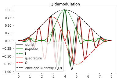
We chose the example signal as following : $a(t)$ is a hanning window, $\omega$ is set so that the central period is one and $\theta$ is a sinusoid that makes one full oscillation : it worth $\pi /2$ at $t = 2$, 0 at $t=4$ and $-\pi/2$ at t=6. We can see that $I$ and $Q$ behaves as some kind of signed envelope for the in-phase and quadrature component. The envelope is perfectly assessed.

Quadrature demodulation

Here a link on how to compute $I$ and $Q$ by mixing and filtering the signal. The idea is to mix (multiply) the signal with two oscillator shifted by 90° (aka $cos$ and $sin$). This translate the frequency spectrum but also generate mirrored components that need to be low-pass filtered. This is achieved with some analog filters.

Analytic signal

I won't define the Hilbert transform. I will only use one of its proprieties : it acts as an 90° phase shifter :

$\mathcal{H}(cos) = sin$

$s(t) = a(t) cos(\phi (t) )$

$\mathcal{H}(s)(t) = a(t) sin(\phi (t) )$

The analytical signal is just an extension of the signal in the complex domain :

$\hat{s} = s + j\mathcal{H}(s) = a(t) e^{j\phi(t)}$

The norm of the analytic signal is $a(t)$ and the argument is $\phi(t)$. Note that this time this representation doesn't imply to provide a central frequency.

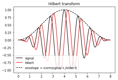
The 90° phase shifter propriety of the Hilbert transform is easy to see here. Again the envelope is perfectly assessed

Hilbert Transform

This transformation can be achieved by two FFT. It consists in suppressing the negative frequency. In practice it can be approximated by some FIR filters. Here a link on how to do that.

From the Analytic to the $IQ$ representation

Those two representations seem really close, can we derive one from the other ? Indeed it is possible. If we start from the analytic signal and by providing the central frequency we can derive a $IQ$ representation by :

$IQ(t) = \hat{s}(t) e^{-j\omega t}$

Hence both processing can be used to produce any of the two representations thank to this formula. Here we can easily see that $IQ$ representation depends on the $\omega$ chosen where $\hat{s}$ doesn't. Let's play with that : using the former formula we compute different $IQ$ representations with different $\omega$.

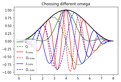
Choosing the original $\omega$ provides the same result as before. Choosing omega 50% bigger or smaller changes the representation but doesn't change the enveloppe (black solid line). In theory choosing any $\omega$ works but in practice, computing $I$ and $Q$ by mixing the signal with a sinusoid and performing low pass filtering constrains the choice of this latter. Note that if we choose $\omega=0$ we come back to the analytic signal. Choosing the right $\omega$ ensures us that $I$ and $Q$ spectrum will be as low in frequency as possible as we can see in this example : the green lines variate more slowly than the red and blue lines an thus is a more relevant representation.

Comparing IQ and analytic representation

Finally the $IQ$ representation is noting else than a down mixed version of the analytic signal. Down mixing is multiplying the signal with an oscillator of frequency $\omega$. In the Fourier space, this corresponds to a translation. Applying it in the real domain generates mirrored replicas of the spectrum that needs to be filtered out but on the complex analytic signal those don't appear.

At first the analytic signal seems more powerful. It doesn't imply to choose a centered frequency. But the $IQ$ representation as it is down mixed has the great advantage to be at a lower frequency hence requiring to be sampled at a lower rate. This reduces memory storage and computation required in the following processing stage. If only the envelope is retained, both representations are equivalent as an intermediate step to perform the envelope but if the phase has to be retained, the $IQ$ representation offers a natural way to store both the envelope and the phase information. Retaining the signal as the couple amplitude $a(t)$ and angle $\phi(t)$ also works but angles are not allways easy to manipulate as they often need to be wrapped/unwrap for further processing.

Comparing Hilbert Transform and $IQ$ demodulation

If it has to be performed in the analog domain, $IQ$ demodulation is the way to go. In the digital domain, Hilbert transform has the great advantage that it can be performed by a simple couple of FIR filters, to be broadband and it doesn't imply to choose a centered frequency $\omega$. The $IQ$ demodulation can be performed by simulating the analog filter or by a smart approach called quadrature sampling. Here a link on this smart approach. Choosing the right implementation depends on the hardware architecture and functionality needed but Hilbert approach is more common those days.

Conclusion

Those two representations are really close. There is some confusion about what is called $I$ and $Q$. They can be defined as above but sometimes also as the in-phase signal and the quadrature components we evoked earlier. The quadrature demodulation comes from the analog world and is performed by mixing the signal with the output of an oscillator at a chosen frequency. Hence it implies choosing a parameter. The Hilbert Transform is parameter free but can't be performed in the analog domain. If no Doppler processing is implied both representations are equivalent. In the contrary, $IQ$ is the natural way of storing both the amplitude and phase information at lower sample rate. Switching from one representation to the other is easy so both Hilbert transform and quadrature demodulation can be use to obtain both representation. Both have been used in high quality ultrasound scanners.

Further Reading

To better understand frequency mixing and quadrature demodulation, I recommend reading this paper:

Quadrature Signals: Complex, But Not Complicated by Richard Lyons

Annex : Code used to generate the plots

import numpy as np
from scipy import signal as sp
from matplotlib import pyplot as plt

# Constants
N = 1000 # number of samples
omega = 2*np.pi # pulsation
T = 2*np.pi/omega # period
cycles = 8   # cycles of carrier wave

# Compute signals
t = np.linspace(0,T*cycles,N) # time
a = np.hanning(N) # envelope
theta = np.pi/2*np.sin(2*np.pi*t/np.max(t)) # phase
phi = omega*t + theta # instantaneous phase
x = a*np.cos(phi) # signal
inphase = a*np.cos(omega*t)*np.cos(theta) # in-phase component
quadrature = -a*np.sin(omega*t)*np.sin(theta) # quadrature component
I = a*np.cos(theta) # I
Q = a*np.sin(theta) # Q
H = np.imag(sp.hilbert(x)) # Hilbert Transform

# IQ demodulation
plt.figure(1)
plt.title('IQ demodulation')
plt.plot(t,x,'k',label='signal')
plt.plot(t,inphase,'g',label='in-phase')
plt.plot(t,I,'g--',label='I')
plt.plot(t,quadrature,'r',label='quadrature')
plt.plot(t,Q,'r--',label='Q')
plt.plot(t,np.abs(I+1j*Q),'k--',label='envelope = $norm(I+j Q)$')
plt.legend(loc='lower left')
plt.show()

# Hilber transform
plt.figure(2)
plt.title('Hilbert transform')
plt.plot(t,x,'k',label='signal')
plt.plot(t,H,'r',label='hibert')
plt.plot(t,np.abs(x + 1j*H),'k--',label='envelope = $norm(signal+j hilbert)$')
plt.legend(loc='lower left')
plt.show()

# Choosing different omega
analytic = x + 1j*H
IQ = analytic * np.exp(-1j*omega*t)
IQplus = analytic * np.exp(-1.50j*omega*t)
IQminus = analytic * np.exp(-0.50j*omega*t)

plt.figure(3)
plt.title('Choosing different omega')
plt.plot(t,np.real(IQ),'g',label='I')
plt.plot(t,np.imag(IQ),'g--',label='Q')
plt.plot(t,np.abs(IQ),'k')
plt.plot(t,np.real(IQplus),'r',label='$I_{+50\%}$')
plt.plot(t,np.imag(IQplus),'r--',label='$Q_{+50\%}$')
plt.plot(t,np.abs(IQplus),'k')
plt.plot(t,np.real(IQminus),'b',label='$I_{-50\%}$')
plt.plot(t,np.imag(IQminus),'b--',label='$Q_{-50\%}$')
plt.plot(t,np.abs(IQminus),'k')
plt.legend(loc='lower left')
plt.show()

List of authors

Alister Trabattoni